Monte Carlo#
Now that you have written your own MD code, you have a recipe for evaluating thermodynamic properties of systems in the microcanonical ensemble. We used MD simulations to sample configurations from that ensemble and, since they all had the same probability, we took their arithmetic mean to calculate ensemble averages. But what would you do if you wanted to sample the canonical ensemble? You would have to evaluate Equation (38), in which each configuration has a different weight. Effectively, this also means evaluating very high-dimensional integrals, since \(\textbf x\) is of dimension \(6N\) where \(N\) is the number of atoms. Here, we will learn about the difficulties of calculating such integrals and of an ingenious algorithm to overcome them.
Evaluation of high-dimensional integrals#
As we have seen, the expectation values we encounter in statistical mechanics are of the form
where
is a positive, normalized phase space probability density. From now, we will consider the canonical ensemble, for which \(\mathcal{F}(\mathcal{H} (\textbf{x})) = e^{-\beta \mathcal H (\textbf x)}\).
How could we evaluate these expectation values in practice? One way is to sample \(a(\textbf{x}_j)\) on a multi-dimensional grid, multiplying each one of the samples by its probability and doing the integration by quadrature,
However, this is very, very expensive and the algorithm scales exponentially with the particles. Why? Because we need to evaluate a \(6N\) dimensional integral on a grid.
Admittedly, if the property we are interested in does not depend on the momenta, i.e. \(a(\textbf{x}_j) = a(\textbf{r}_j)\), then the integration over \(\textbf p\) can be done analytically to obtain,
Nevertheless, we remain with a \(3N\) dimensional integral. To evaluate it, even if we divide each spatial dimension for every particle into only 10 grid points, we would need to sum over \(N_g = 10^{3N}\) points to evaluate the integral. This is completely prohibitive already for a very small number of particles. Monte Carlo is a clever way to evaluate such integrals without resorting to quadrature. Moreover, Monte Carlo is a conceptually different approach for sampling equilibrium distribution functions that does not rely on the dynamics in time of the system to generate the configurations (like MD).
Uniform random sampling#
A solution to this problem was invented by Ulam and Metropolis in 1949. Their ingenious idea was to use random numbers to evaluate multidimensional integrals instead of a quadrature on a grid. They showed that using their approach, it is possible to evaluate integrals using a much smaller number of samples than the exponentially growing number of grid points. Their idea was to choose a known reference volume in space that bounds the (irregular volume) we wish to calculate. Then, we sample random points uniformly distributed in the reference volume. We count the number of samples that lie within the irregular volume we wish to calculate. The ratio of this number to the total number of samples, multiplied by the reference volume is an estimate of the irregular volume,
For example, to evaluate the area of a two-dimensional disk with radius \(R=1\) in the first quadrant, we need to solve the integral
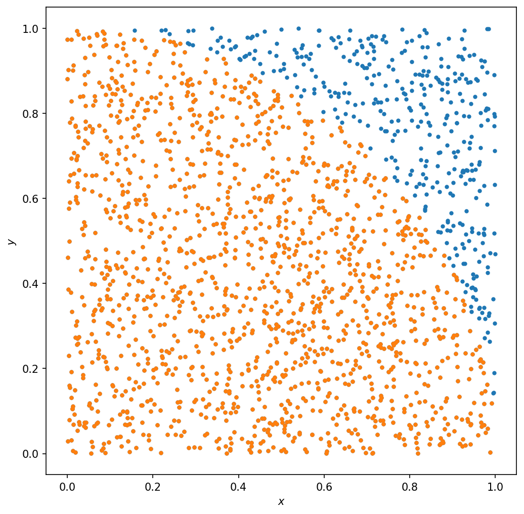
Instead, we choose a reference square of unit side length that bounds the unit circle and evaluate the integral numerically using MC uniform sampling. Below we demonstrate this method and evaluate the area/volume of a ball in two and three dimensions, using both quadrature and Monte Carlo uniform sampling. To treat the two methods on equal footing, we make sure to use the same number of function evaluations and compare the obtained accuracy. We show that for two dimensions, quadrature is more accurate than MC sampling. But already for three dimensions, MC is more accurate by an order of magnitude. MC is also much faster than quadrature for three dimensions.
#imports
import numpy as np
import math
import matplotlib.pyplot as plt
import time
from scipy import integrate, special

#Radius of unit sphere
R = 1
#2D quadrature
func = lambda x,y: x**2 + y**2 <= R**2
tstart = time.time()
data = integrate.nquad(func, [[0,R], [0,R]], full_output=True)
tend = time.time()
print(data)
print("Time in seconds: ", tend-tstart)
(0.7854453780175082, 6.043574189984469e-06, {'neval': 1888215})
Time in seconds:  0.6616497039794922
#3D quadrature
func = lambda x,y,z: x**2 + y**2 + z**2 <= R**2
integrate.nquad(func, [[0,R], [0,R], [0,R]], full_output=True)
(0.5236018744846193, 0.0001344051879086777, {'neval': 1839958785})
def evalSphereVol(d, Nsamples, M):
    rng = np.random.default_rng()

    res = np.array([])
    for seed in range(M):

        #generate random samples
        p = rng.uniform(0,R, size= (d,Nsamples))

        #count how many are inside the n-ball
        inside = ((p**2).sum(axis=0) <= R**2).sum()
        V0 = R**d
        res = np.append(res, inside/Nsamples*V0)

    return res, p
#2D MC uniform sampling
d = 2

Nsamples = 188822
M=10

tstart = time.time()

res, p = evalSphereVol(d, Nsamples, M)

tend = time.time()
print("Time in seconds: ", tend-tstart)

print("Mean = " + str(res.mean()) )
print("BSE = " + str(res.std()/np.sqrt(M)) )

#volume of d-ball in first quadrant
voln = math.pi**(d/2) * R**d / special.gamma(d/2 + 1) / 2**d
print( "Expected = " +  str(voln) )

print("neval = " + str(Nsamples*M) )
Time in seconds:  0.030365467071533203
Mean = 0.7859364904513244
BSE = 0.00026968770186146517
Expected = 0.7853981633974483
neval = 1888220
plt.figure(1, figsize=(8,8), dpi=150)
plt.xlabel(r"$x$")
plt.ylabel(r"$y$")

lessp = p[:,0:-1:100]
idx = lessp[0,:]**2 + lessp[1,:]**2 <= R**2

plt.plot(lessp[0,:],lessp[1,:],'.')
plt.plot(lessp[0,idx],lessp[1,idx],'.')
[<matplotlib.lines.Line2D at 0x7fce8ff72e20>]
#3D MC uniform sampling
d = 3
Nsamples = 183995879
M=10

tstart = time.time()

res, p = evalSphereVol( d, Nsamples, M)

tend = time.time()
print("Time in seconds: ", tend-tstart)

print("Mean = " + str(res.mean()) )
print("BSE = " + str(res.std()/np.sqrt(M)) )

#volume of d-ball in first quadrant
voln = math.pi**(d/2) * R**d / special.gamma(d/2 + 1) / 2**d
print( "Expected = " +  str(voln) )

print("neval = " + str(Nsamples*M) )
Time in seconds:  35.81044626235962
Mean = 0.5235936452685443
BSE = 1.2164749650874706e-05
Expected = 0.5235987755982989
neval = 1839958790
The Central Limit Theorem#
We have just established that random (uniform) sampling could be very helpful for evaluating multi-dimensional integrals, in comparison to numerical quadrature. But there are situations in which uniform sampling could be highly wasteful too. For example, when \(f(\textbf x)\) is localized in a small volume in the \(3N\) dimensional space. In that case, many of our uniform samples will not be counted when evaluating the integral.
Note that this is not the case for the example of the n-ball above. For the n-ball, the volume grows like \(\sim R^d\) where \(d\) is the number of spatial dimensions. We sample uniformly in an \(d\)-dimensional cube, whose volume also scales the same. This means that the ratio of the two volumes does not depend on \(d\).
For the problematic, localized case, can we do better than uniform sampling? Yes! If we know how to generate samples that are already distributed according to \(f(\textbf x)\).
At this point, we will assume that we have an algorithm for obtaining a set of \(M\) independent samples (configurations of the system) \(\textbf x_1 ,..., \textbf x_M\) that are all identically distributed according to \(f(\textbf x)\) with some mean \(\langle a \rangle_f\) and variance \(\sigma^2 = \langle a^2 \rangle_f - \langle a \rangle_f^2\). This is by no means a trivial task. It is straightforward only for simple distributions and the form of Monte Carlo that we will study next was designed to address exactly this problem. But, for now, we will simply assume such an algorithm exists. If that is the case, we can then evaluate \(a(\textbf{x}_j)\) for each sample.
The central limit theorem (CLT) ensures that if we consider the simple arithmetic mean of the samples as a random variable,
It will be normally distributed with the same mean \( \langle a \rangle_f \) as the samples \( \textbf{x}_j \) and a variance
In other words, the CLT guarantees that the arithmetic mean of the samples converges to the ensemble average of \(A\) in the limit \(M \to \infty\), because its variance from the mean decays like \(M^{-1}\). Note that the CLT does not assume a specific form of the distribution \(f(\textbf{x})\). This is very powerful, it means that even when our sampling algorithm (dynamic or not) provides samples from a nonuniform distribution, the arithmetic mean will still converge to the true expectation value. An important outcome is that we can use the simple arithmetic mean of the samples to calculate expectation values for the canonical ensemble, just like in the NVE ensemble, as long as we can generate samples from the desired distribution.
However, that is exactly where things get tricky! We know how to generate random samples only from relatively simple probability distributions (Gaussian, uniform, exponential, see others here).
There are two solutions to this problem: 1) Use a different distribution, \(h(\textbf x)\), that is simple enough to be sampled directly and resembles \(f(\textbf x)\) better than a uniform distribution. 2) Generate samples consecutively (and not altogether at random as we did above) in a process that is sure to converge to the distribution \(f(\textbf x)\). The first solution is called importance sampling, which we describe first. The second solution, called the Metropolis Monte Carlo or Markov Chain Monte Carlo, will be discussed in the next section.
Importance Sampling#
We can use the CLT even if we do not know how to sample from \(f(\textbf x)\) directly, but know how to sample a different distribution, \(h(\textbf x)\), that has much more substantial overlap with \(f(\textbf x)\) than the uniform distribution. Since \(h(\textbf x)\) is a positive, normalized probability density, we rewrite Equation (60) as
where \(w(\textbf x) = f(\textbf x) / h(\textbf x)\) is the weight we need associate with every configuration sampled from \(h(\textbf x)\) to obtain the expectation value we are really interested in, Equation (60). As a result, this procedure is also often called reweighting.
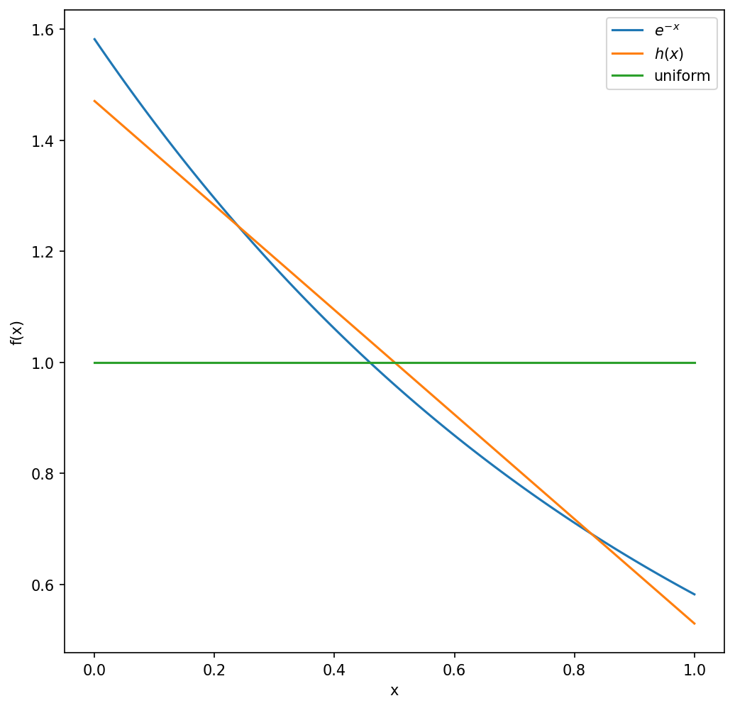
Below we show an example from the book by Tuckerman that uses importance sampling to evaluate the integral
If we sample \(x\) uniformly, we get a good estimate of the mean after 1000 random samples. But the error is an order of magnitude smaller if we use importance sampling with
while choosing \(a\) to have the higest similarity between \(h(x)\) and \(e^{-x}\). The similarity is measured using a function called the Kullback-Leibler (KL) divergence, the optimal value is found to be \(a=0.64\).
Active learning
Show that \(h(x)\) given above is a positive and normalized probability density in the range [0,1].
Solution
Ng=100; a=0.64

plt.figure(figsize=(8,8), dpi=150)
xg = np.linspace(0,1,Ng)

p = np.exp( -xg ) / np.trapz( x=xg, y=np.exp(-xg) )
q = ( 1 - a*xg )/( 1 - a/2 )
q2 = np.ones(Ng)

print( "KL divergence h(x) = " + str( np.sum( special.rel_entr(q,p) ) ) )
print( "KL divergence uniform = " + str( np.sum( special.rel_entr(q2,p) ) ) )

plt.plot( xg, p, label = r"$e^{-x}$" )
plt.plot( xg, q, label = r"$h(x)$" )
plt.plot( xg, q2, label = "uniform" )
plt.legend()
plt.xlabel(r"x")
plt.ylabel(r"f(x)")
KL divergence h(x) = -0.011662666832944757
KL divergence uniform = 4.133335709606822
Text(0, 0.5, 'f(x)')
How do we sample from \(h(x)\)? If we have \(\xi\), which is sampled from a uniform distribution between \([0,1]\), other distributions \(h(x)\) in the same range can be obtained if we can solve the inverse equation
The solution \(x\) will be then distributed according to \(h(x)\). We see below that for a simple linear distribution this becomes a second-order root search problem. For more complicated distributions, the resulting equations are too difficult to solve.
Active learning
Show that the solution of the above inverse equation is
Solution
The integral leads to
Which can be rearranged as a second order equation
whose solution is the expression given above. Bonus: What happened to the other root?
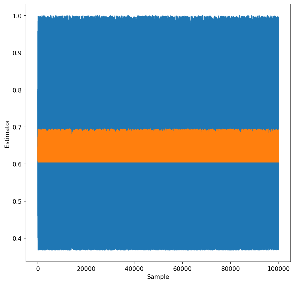
The advantage of importance sampling can be also seen in the figure below, showing the value of the estimator, \(e^{-x}\) or \(e^{-x}/h(x)\), for the generated random samples. It is clear that the standard deviation of the latter is much smaller. Note that if we would have chosen \(a=1\), the sampling would actually be worse that for the case of uniform sampling.
def sampleh(p, a=1):

    newp = ( 1 - np.sqrt(1 - ( 1 - a/2 ) * 2 * a * p) ) / a
    h = (1 - a * newp) / ( 1 - a/2 )
    #plt.hist(p[1,:-1:100], bins=20)
    return newp,h

Nsamples = 100000
M=10

res = np.array([])
res_IS = np.array([])
for seed in range(M):

    rng = np.random.default_rng()

    #generate random samples
    p = rng.uniform(0,R, size= Nsamples)
    expp = np.exp(-p)

    #append result for this realization
    res = np.append(res, np.mean(expp))

    #Sample from h instead
    newp, h = sampleh(p, a=0.64)

    #Evaluate new estimator e^-x/h(x)
    expp_h = np.exp(-newp)/h

    #append result for this realization
    res_IS = np.append(res_IS, np.mean(expp_h))

print("uniform mean = " + str(res.mean()) )
print("uniform BSE = " + str(res.std()/np.sqrt(M)) )

print("IS mean = " + str(res_IS.mean()) )
print("IS BSE = " + str(res_IS.std()/np.sqrt(M)) )

print("expected = 0.632120558829")

plt.figure(figsize=(8,8), dpi=150)
plt.plot(expp)
plt.plot(expp_h)
plt.xlabel(r"Sample")
plt.ylabel(r"Estimator")
uniform mean = 0.6322484133201973
uniform BSE = 0.0002341326057815266
IS mean = 0.6321353195266276
IS BSE = 2.5306811085860125e-05
expected = 0.632120558829
Text(0, 0.5, 'Estimator')
Finally, we note that importance sampling is useful not only when we do not know how to sample \(f(\textbf x)\). For example, when \(a(\textbf x)\) is highly oscillatory, with both negative and positive contributions, such that its expectation value results from the near-cancellation of the positive and negative terms. We do not go into detail here, but a judicious choice of \(h(\textbf x)\) could significantly improve convergence in such difficult cases.
Metropolis Monte Carlo and detailed balance#
We already saw that if we have a way to sample \(f(\textbf x)\), we can easily obtain expectation values using importance sampling MC. But it is an unfortunate fact that we have efficient algorithms to sample directly only relatively simple distributions, such as exponential, Gaussian, uniform, etc.
In a seminal paper in 1953, Arianna and Marshall Rosenbluth, Augusta and Edward Teller, and Nicholas Metropolis (sans spouse) developed an algorithm that, instead of obtaining random samples from \(f(\textbf x)\) at once, creates a sequential samples \(\textbf{x}_1, \textbf{x}_2, ...\) that converge to the correct \(f(\textbf x)\), for an arbitrary distribution function! The importance of this result truly could not be overstated. It is perhaps one of the greatest results of the previous century.
The idea at the core of the algorithm is that we need to specify a rule to generate the next sample \(\textbf{x}_{i+1}\) from the current sample \(\textbf{x}_i\). A sequence of samples that is generated based on information solely from the previous step is called a Markov chain. We denote the probability of obtaining a sample \(\textbf x\) from some other sample \(\textbf y\) as \(R(\textbf x | \textbf y)\). For this probability to be a valid rule for generating a Markov chain, it must satisfy a condition called detailed balance,
where \(R(\textbf x | \textbf y) f(\textbf y)\) is called the a priori probability of moving from \(\textbf y\) to \(\textbf x\), which is just the probability to move from \(\textbf y\) to \(\textbf x\), given that the system was already in \(\textbf y\). Detailed balance is important, because it guarantees that the Markov chain is microscopically reversible, which can be shown to be an important property of thermodynamic equilibrium. It effectively ensures that if, during the Markov chain, we reach the distribution \(f(\textbf x)\), it will be stationary.
After a move is generated, we must decide whether to accept it or not.
The Metropolis MC algorithm states a rule for proposing moves, which we denote as \(T(\textbf x | \textbf y)\), which has to be normalized,
and a probability that the move is accepted, which is denoted as \(A(\textbf x | \textbf y)\). Then the probability to move from \(\textbf y\) to \(\textbf x\) is given by the product of the probability of suggesting such a move, times the acceptance probability, i.e.
Inserting this equation into the detailed balance conditions, Equation (68) we get
where
Now, suppose \(A(\textbf x | \textbf y)=1\) and the move from \(\textbf y\) to \(\textbf x\) is favorable, then \(A(\textbf y | \textbf x) < 1\) and therefore \(r(\textbf x | \textbf y) > 1\). However, if \(A(\textbf x | \textbf y)<1\), then \(A(\textbf y | \textbf x) = 1\) is favorable and so \(r(\textbf x | \textbf y) < 1\). We can summarize these findings as
Now all the ingredients for Metropolis MC are ready! Given that the system is at some configuration \(\textbf{x}_k\), we define a probability \(T(\textbf{x}_{k+1} | \textbf{x}_k)\) and suggest a new trial configuration \(\textbf{x}_{k+1}\). Next, based on \(\textbf{x}_{k+1}\) and \(\textbf{x}_k)\), and the probability we want to sample, \(f(\textbf{x}_k)\), we evaluate the ratio \(r(\textbf{x}_{k+1} | \textbf{x}_k)\) using Equation (70). Finally, we accept or reject the move based on the criterion in Equation (71). The final step is done in practice in the following way: If \(r(\textbf{x}_{k+1} | \textbf{x}_k) \ge 1\) the move is accepted. If it is smaller than 1, the step is accepted with probability \(r(\textbf{x}_{k+1} | \textbf{x}_k)\), i.e., a random number \(\xi\) is sampled from a uniform distribution between \([0,1]\). If \(r(\textbf{x}_k | \textbf{x}_{k+1}) \gt \xi \), the move is accepted. Otherwise, the move is rejected.
MC moves and acceptance ratio#
A simple, but rather useful, MC move is a translation with uniform probability from \(\textbf{y}\) to any point \(\textbf x\) within a box of side length \(2\Delta\) centered around y. The volume of the box is denoted by \(V_{\Delta}\). The trial probability, our rule for making moves, is then given by
This probability is properly normalized, and it is also symmetric, i.e. \(T(\textbf x | \textbf y) = T(\textbf y | \textbf x) \). As a result, the acceptance criterion of Equation (71) becomes
Now, if we wish to sample the canonical ensemble, the probability is \(f(\textbf{r}) \propto e^{- \beta U(\textbf{r}) }\), giving an acceptance probability
This means that if the new proposed step has a lower potential energy, the move is accepted. If the potential energy of the new configuration is high, though, it is accepted with a probability that is the ratio of Boltzmann factors.
A point of emphasis here is that the probability of accepting a new move in the canonical ensemble is that the new energy would not be very different than the previous energy. Since the energy is an extensive quantity, changing randomly the positions of all of the particles at once, would result in a massive energy change. Thus, we cannot move all particles together, like in MD simulations. The solution to this problem is to select randomly a single atom \(i\) to move, and change its coordinates in the following manner:
where \(\zeta\) is a vector of three independent uniform random numbers in the range \([-1,1]\). Repeating this process \(N\) times, where \(N\) is the number of atoms in the system, is called a MC pass. Notice that this does not necessarily mean that all atoms have been moved since we choose the atoms randomly.
Two final comments are in order: First, when we need to evaluate the difference in potential energies after moving a single particle at random, we do not need to compute all of the potential energy from scratch. That is very expensive, and we should update only the interactions of the chosen particle. Second, that the parameter \(\Delta\) has an important effect on the percentage of MC steps that will be accepted, which is called the acceptance ratio. If \(\Delta\) is too large, the change in potential energy will be large, and many moves will be rejected. If it is too small, all moves might be accepted but we will not explore all of phase space efficiently. Therefore, a rule of thumb is to use an acceptance ratio between \(20 \% - 50 \%\).
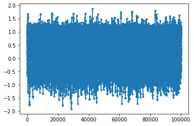
Demo - sampling 1D arbitrary distributions#
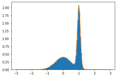
In the demo below, we use Metropolis MC to sample from a bimodal probability distribution that would not have been simple to sample otherwise. Already in this 1D example, we see the utility of the MC approach!
#Generic probability distribution
def evalf(x):
    mu1 = 1
    sigma1 = 0.1
    g1 = np.exp(-0.5*(x-mu1)**2/(sigma1**2))/np.sqrt(2*math.pi)/sigma1

    mu2 = 0
    sigma2 = 0.5
    g2 = np.exp(-0.5*(x-mu2)**2/(sigma2**2))/np.sqrt(2*math.pi)/sigma2

    return (g1+g2)/2 #evaluated normalization with trapz

#number of MC steps
Nsteps = 100000

#maximal step size
delta = 0.7

rng = np.random.default_rng()

#initial position
xn = 1

x = np.array([])

x = np.append(x, xn)

#for acceptance ratio
accept = 0

for step in range(Nsteps):

    xnp1 = xn + delta * np.random.uniform(low=-1.0, high=1.0)

    ratio = np.divide(evalf(xnp1),evalf(xn))

    xsi = np.random.uniform()

    if ratio < xsi:
        x = np.append(x, xn)
    else:
        x = np.append(x, xnp1)
        xn = xnp1
        accept += 1

plt.hist(x[100:], bins=100, range=(-3,3), density=True)
xg = np.linspace(-3,3,1000)
plt.plot(xg, evalf(xg))
print("normalization: ",np.trapz(evalf(xg), xg))

plt.figure()
plt.plot(x,'.-')
print("Acceptance ratio: ",accept/Nsteps)
normalization:  0.9999999990129743
Acceptance ratio:  0.53599
Sampling other distributions#
We have seen how to generate configurations according to an arbitrary probability density function using the Metropolis algorithm. We also saw in Equation (72) the expression for the acceptance probability for the canonical ensemble. But the great merit of MC simulations is that it is usually much easier to extend them to other ensembles than MD simulations (although that is also possible!).
For example, if we are interested in the isothermal-isobaric ensemble, in which the number of particles \(N\), the pressure \(P\), and the temperature \(T\) are fixed (the \(NPT\) ensemble), we can do so rather easily. There are only two changes that need to be made to the algorithm that samples from the canonical ensemble: First, we need a move to change the volume of the system,
where \(\zeta\) is a random variable just like in Equation (73), and \(\Delta_V\) is the maximal allowed change in volume.
Secondly, each time the volume changes, the particle coordinates must be scaled accordingly by
and the potential energy needs to be re-evaluated.
Finally, since in this ensemble \(f(\textbf x,V) \propto V^N e^{-\beta ( U(\textbf x) + PV) }\) the volume moves are accepted with probability
where
Much more elaborate MC moves can be designed. As long as they obey detailed balance, they are legitimate and can be used to sample various distributions. One interesting example is the case where the potential energy has many local minima separated by high barriers. In that case, standard MC translation moves will not work anymore and the system will be trapped in one of the local minima. One solution to this problem is called parallel tempering or replica exchange, in which several replicas of the system are simulated using standard MC simulations but at increasing temperatures.
We are interested in sampling the system at the lowest temperature but systems are higher temperatures will cross the energy barriers more easily. Therefore, every several MC passes, a pair of neighboring replicas are chosen and a move is attempted to switch their particle coordinates. For example, if before the move the system at temperature \(\beta\) was in configuration \(\textbf x\) while the system in temperature \(\beta'\) was in configuration \(\textbf y\), one can show that in that the acceptance probability should be
where \(\delta = \left( \beta' - \beta \right) \left[ U(\textbf y) - U(\textbf x) \right]\).
In one of the final projects, you will implement such a replica exchange MC simulation and compare it with alternative algorithms to overcome high energy barriers that are based on MD simulations.
Proof that \(f(x)\) is a stationary point of Metropolis MC#
We follow the proof that is presented in the Book by Tuckerman. At every iteration of the Markov chain/Metropolis algorithm, the points \(\textbf{x}_k\) are distributed according to some function \(\pi_k(\textbf x)\). We wish to show that if the algorithm reached a point in which \(\pi_k(\textbf x) = f(\textbf x)\), all following steps will be distributed according to \(f(\textbf x)\). In other words, we wish to show that \(f(x)\) is a stationary point of the Metropolis algorithm.
We will use induction to prove that is the case. We will assume that at some arbitrary MC step \(k\), \(\pi_k(\textbf x) = f(\textbf x)\), then we will derive the expression for \(\pi_{k+1}(\textbf x)\), the distribution in the next MC step, and we will show that it is also equal to \(f(\textbf x)\).
The probability to be at point \(\textbf x\) at step \(k+1\), \(\pi_{k+1}(\textbf x)\), has two contributions: First, from moves that started in other points \(\textbf y\), proposed \(\textbf x\) as a new configuration and were accepted. The term is given by the probability to be at \(\textbf y\) in the previous step, \(\pi_{k}(\textbf y)\), times the probability that \(\textbf x\) will be proposed as the next move if we are at \(\textbf y\), \(T(\textbf x | \textbf y)\), times the probability that the move will be accepted, \(A(\textbf x | \textbf y)\). The final expression for this first contribution is then given by integrating over all the possible initial \(\textbf y\),
The second contribution includes moves that started at \(\textbf x\), proposed some new step \(\textbf y\), and were rejected. This term is equal to the probability to be at \(\textbf x\) in the previous step, \(\pi_{k}(\textbf x)\), time the probability that \(\textbf y\) will be proposed as the next step, \(T(\textbf y | \textbf x)\), times the probability that the move will be rejected, \(1 - A(\textbf y | \textbf x)\). The final expression is given by integrating over all possible moves \(\textbf y\),
Combining these two contributions, we get
Now, we assume that \(\pi_k(\textbf x) = f(\textbf x)\) and rearrange Equation (79) to get
The first integral vanishes due to detailed balance, Equation (68), and in the second term we can take \(f(\textbf x)\) out of the integral. Finally, since \(T(\textbf y | \textbf x)\) is normalized (see Equation (69)), we get
which completes the proof.
Combining MD and MC for canonical time correlation functions#
In the last section of the MD chapter, we discussed how to evaluate various observables. We looked at properties like the kinetic energy (Equation (56)), potential energy (e.g., Equation (54)), and also at structural properties like the density (see Equation (57)). In your first numerical exercise, you even evaluated spatial correlations by looking at the radial distribution function (AKA pair correlation function). The same estimators can be used in MC simulations to evaluate expectation values in the canonical ensemble. You will do just that in your second numerical exercise!
But we also mentioned special observables, called equilibrium time-correlation functions, that were defined in Equation (58). You might recall that their special importance came from the fluctuation dissipation theorem which states that the response of a system to a small time-dependent perturbation, driving the system out of equilibrium, is determined by equilibrium time-correlation functions. In other words, the response, as measured by transport properties (diffusion, thermal/electric conductivity, reaction rate, etc.), is determined by the fluctuations of equilibrium time correlation functions.
Of the methods we have discussed in the course, time correlation functions can only be evaluated by doing MD simulations. The reason we cannot evaluate them using MC simulations is that the steps in the Metropolis algorithm are determined by a random process - they store no information about the dynamics in time of the system.
On the other hand, our MD simulations only allowed us to evaluate expectation values in the microcanonical ensemble. But most transport properties are measured in experiments at constant temperature, not energy! To the rescue comes the combination of MC and MD.
To evaluate time correlation functions in the canonical ensemble, we can perform one long MC simulation, which will converge to sampling configurations from the Boltzmann distribution. Once it is converged, we can take a sample every few hundred steps and, from each one, generate regular MD trajectories at constant energies to determine the time correlation function for this particular energy. Taking the average over all of the trajectories (initial conditions) will give the desired time correlation functions in the canonical ensemble. In your second exercise you will do this to evaluate the self-diffusion coefficient of Argon at various temperatures.
Error estimation#
Finally, assuming we have managed to evaluate some expectation values, how accurate are they? What is the statistical uncertainty of our results? An estimate of the statistical error can be obtained by using the central limit theorem again. Loosely speaking, it states that, under certain conditions, the means of samples of independent random variables are normally distributed. This is true even if the original variables are not normally distributed.
Practically, it means that if we have some property \(A\) which is not normally distributed, as is often the case in MD/MC simulations, if we sample it many times, divide the samples into \(M\) equal blocks, and then evaluate the mean for each block, \(\langle A \rangle_m\) where \(m=1,...,M\) - those means follow a normal distribution. Why is it important? Because if we know that the means are normally distributed, we can evaluate the standard error on the averages from,
where \(\sigma_A^2\) is the variance between the means of the different blocks,
and \(\langle A \rangle\) is the average from the entire simulation data, as in Equation (55). As we said previously, this analysis can be used in any ensemble, because the means always distribute normally.
The only question that remains is - how do we choose the number of blocks \(M\)? For this analysis to be valid, the different blocks have to generate statistically independent samples of the means. How do we know that the blocks are spaced enough so that this is the case? It turns out, that the autocorrelation function of the observable is the answer. The autocorrelation function starts from a value of \(\langle A^2 \rangle\) and decays towards zero. The time it takes to decay it called the autocorrelation time and it effectively determines how long it takes for the system to forget all past correlations so that new samples are independent from the initial ones. Thus, we need to choose the block length to be larger that the autocorrelation time.
Evaluating time correlation functions is quite expensive, so we do not want to do this for every property (although it is a more rigorous approach). How do we evaluate if our samples are correlated or not in practice? We start with very small blocks (very large \(M\)), containing only a few steps each. In this case, many of our block means are highly correlated. Our estimate of the error on the average of the observable from Equation (80) will be very small because we are assuming all of them are statistically independent, which is not true. Then, we increase the block size (decrease \(M\)) and re-calculate the error on the mean. It will increase a little. We repeat this procedure until our estimate of the error on the average has reached a plateau. Then, our estimate of the number of independent samples of the mean during the simulation is equal to the number of blocks we have used. The procedure to determine the statistical uncertainty according to Equation (80) is then reliable.
We note that this analysis is required if we want to evaluate the statistical error on expectation values that were evaluated in a single simulation. If we have enough time and computational power, we can always resort to doing several independent simulations, by sampling different initial conditions, and simply treat each simulation as an independent block in the error analysis.